Two years of shelf monitoring: a map of the CV pipeline

2025-12-16 · engineering

A supermarket knows its receipts, its deliveries and its foot traffic. What is on the shelf right now is a blank. Receipts show what sold and stay silent on what is left. The delivery system shows the stockroom, while a person moves goods to the floor at their own pace. Ceiling CCTV sees trolleys, and a can of cola behind fridge glass ten meters away stays invisible.

Know the state of every shelf in real time and three things open up: raise on-shelf availability, trigger restocking by item, and catch layout errors as they happen. On-shelf availability converts straight to revenue: a product missing when a shopper reaches for it sells with probability zero. To collect that signal you need your own cameras on the fixtures and a recognition pipeline behind them.

We built that system over about two years for two grocery chains. It started as a pilot in one convenience store and scaled to two flagship hypermarkets of a national grocery chain. The catalog runs to roughly 20,000 SKUs. A few thousand cameras shoot one frame every 30 minutes into S3. Final accuracy (the share of crops given the right product) sits near 96%.

This is the overview note. It maps the four stages of the pipeline and points to the deep-dive notes for each hard part. If you are reading the series for the first time, start here. This is the computer vision work we do, written up stage by stage.

The pipeline in four stages

Every frame travels the same path: capture, preprocess, detect, classify. The output of the last stage is a product_id per crop, and from there come the on-shelf availability (OSA) numbers, alerts and category analytics.

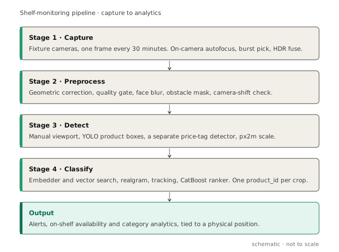
A flow of the shelf-monitoring pipeline across four stages: camera capture, server-side preprocessing, detection of shelves, products and price tags, then classification of each crop into a product id, feeding alerts and on-shelf availability. — The whole system is this pipeline. Each stage hands clean data to the next, and a weak stage caps everything after it.

Stage 1: capture

The input is raw images from cameras on the fixtures. We do not mount the cameras. We do configure them, because what lands in S3 sets the ceiling for everything downstream. This is the same argument as our note on choosing cameras: the lens decides what the model can ever see.

Placement and optics follow the store. Ceiling units look down the aisle, wall units look at the shelf the way a shopper does. Lenses range from wide angle for short bays to longer glass for distant rows.

The cameras shoot on a timer. They wake, connect to our server, take a frame, send it, and sleep. That saves battery on the autonomous units and saves network traffic. For layout control, one frame every 30 minutes is enough.

We push quality up at the camera, where it is cheaper than rescuing a bad frame later. Three tricks live on the device. Autofocus uses the variance of the Laplacian: the camera sweeps the lens, measures sharpness on board, and locks on the peak. A short burst of frames is taken and the sharpest is kept, which guards against motion blur. An HDR pair, one short exposure for highlights and one long for shadows, is fused into a single readable frame. The goal is a frame with no lost data.

Each shot is driven through an API. The server sends focus, exposure, white balance and sharpness before each frame. So a dark corner or a fixed focus distance can be tuned per store.

Stage 2: preprocessing and filtering

When a raw frame reaches the server, cleaning starts before any model sees it.

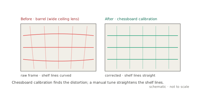
Geometric correction comes first. Wide ceiling lenses bow the image into a barrel. A classic chessboard calibration gives the distortion coefficients. Then a light manual tune in a small Python app straightens the shelf lines for the real mounting angle. The output is a frame with no geometric artifacts.

A raw frame from a wide ceiling lens with shelf lines bowed into a barrel, beside the same frame after chessboard calibration with every line straight. — A wide lens bows the shelf lines. Calibration straightens them before any model runs.

Frame quality control runs next. Despite the on-camera tricks, some frames arrive smeared, blown out or shot through a dirty lens. We measure sharpness on the server and check the histogram for clipping. A frame that fails triggers an off-schedule retake.

Face anonymization is mandatory. A store is a public space, so people land in frame. We detect faces with InsightFace buffalo_l, detection only, with no embeddings and no identity. A strong Gaussian blur from OpenCV covers each box. The step is deliberately blunt: the goal is to remove biometric detail with no risk, before any image is saved. Privacy rules like GDPR are covered, and the CV models lose a distraction they never needed.

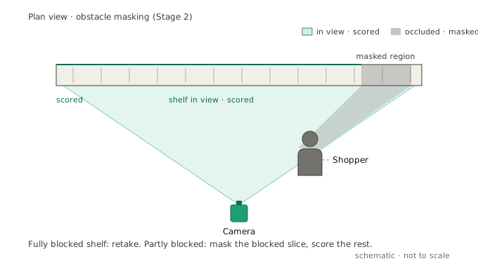
Obstacle detection handles shoppers, trolleys and boxes. A module segments the frame and labels each object: product, person, trolley, stray item. A fully blocked shelf triggers a later retake. A partly blocked shelf is kept, with the blocking region masked so the models do not read a person as part of the display.

Top-down view of a camera looking at a shelf, with a shopper in the aisle casting an occlusion shadow over one slice of the shelf that is masked out, while the rest stays in view. — A shopper blocks one slice of the shelf. That slice is masked; the rest is scored as usual.

Camera-shift control closes the stage. A knock or a tilt moves the view, and then detectors look for the shelf in the wrong place. We compare each frame against a calibrated viewport, a rectangle of interest. A drift either nudges the viewport automatically or alerts a technician. The same triage runs through our note on recognition errors, where most tickets resolve at the lens or the lamp.

Stage 3: detecting shelves, products and price tags

After the filters, the frame is geometrically clean, anonymized, free of obstacles, with a confirmed camera position. Now the vision work begins.

Shelf detection sets the region of interest. We have a shelf detector that finds fixtures automatically. Real stores vary too much for it to drive production. Sometimes only part of a fixture matters, sometimes sections merge, sometimes the zone of interest ignores the physical edge. So production uses manual viewports as the reliable way to set the region. The shelf detector stays on for first-time setup and the shift checks in Stage 2.

Product detection runs on the viewport crop. A current YOLO detector (it draws a box around each item) returns the boxes, and from them we cut crops. Those crops feed Stage 4. Dense displays and products that hide each other are the hard cases here.

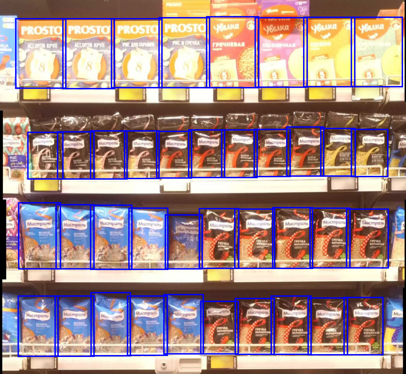
A shelf photo with a YOLO detector's blue boxes around each product. — The detector returns a box per product. Each box becomes a crop for Stage 4.

Price-tag detection runs as its own model. Tags are small, high contrast and structured, so a separate detector suits them. Alongside it we compute px2m, the pixel-to-meter scale, which gives physical sizes and the distance between a tag and a product. That scale matters later for size features and for tag matching.

Stage 4: classifying products

This is the most important and the hardest part. The input is product crops from YOLO. The output is a product_id for each one. Four things make it painful.

A catalog of 20,000 SKUs rules out a plain classifier. The assortment drifts, with new SKUs every week. Crop quality swings with light, angle and occlusion. And many SKUs are visually identical, with the same label across flavors, volumes and weights.

Human labeling is unavoidable. Every client catalog is unique, and no off-the-shelf embedder (a crop-to-vector model) maps a crop to a client product_id on its own. Label too much and it is expensive, too little and quality suffers. Spotting new SKUs early, so they reach labeling first, became its own discipline.

The classifier evolved through four versions. The progression below shows what each one adds. The numbers themselves sit in the deep-dive notes.

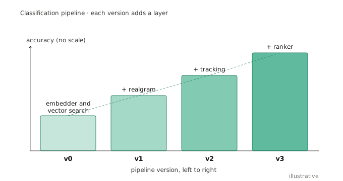
The classifier grew one layer at a time. Visual matching is only the floor; spatial context, cross-frame smoothing and a learned ranker do the rest.

v0: embedder and vector search, around 85%

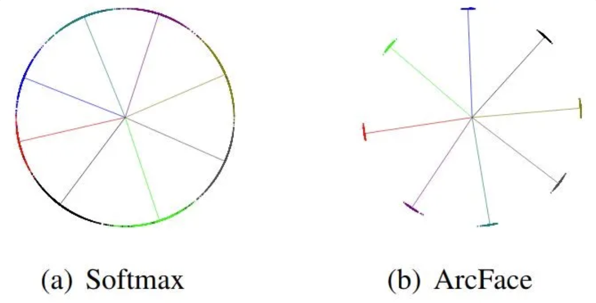
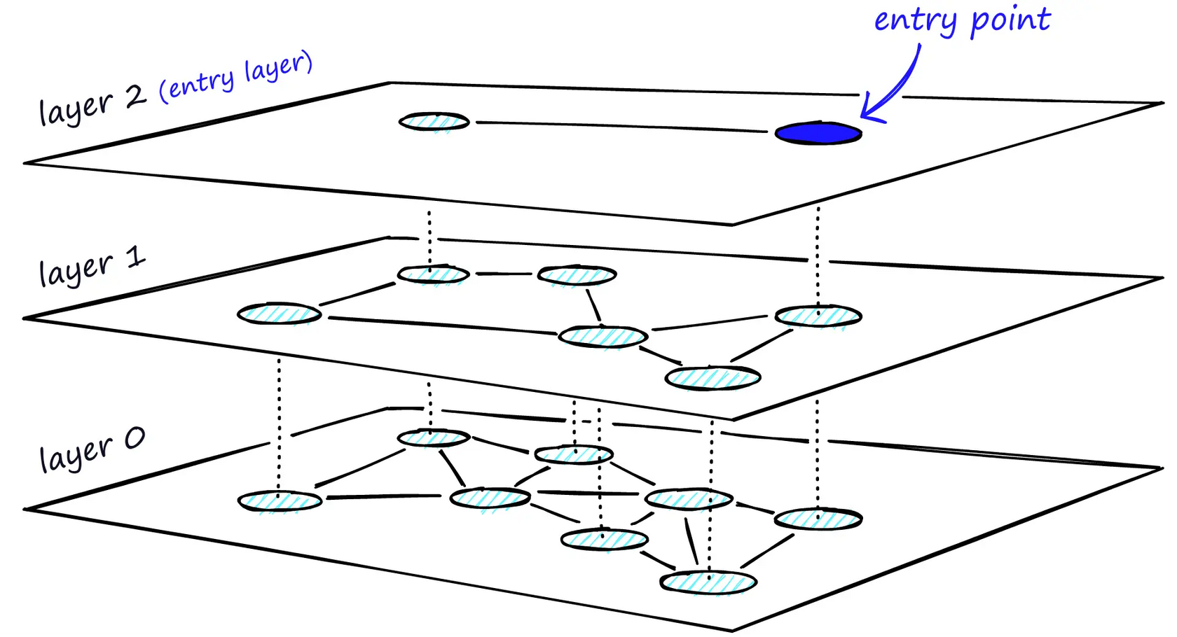
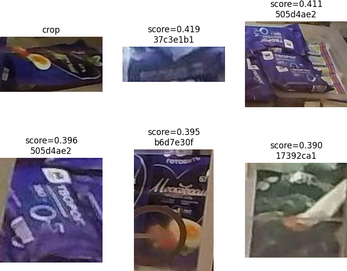
Plain metric learning: train the model so crops of the same product sit close together and different ones sit far apart. A ViT-Base-32 backbone with an ArcFace loss (it spreads look-alikes apart) turns each crop into a 512-dimension vector, its visual fingerprint. Labeled crops go into a Qdrant search space (a database built to find the closest vectors), each with its payload: product_id, store, category. An unlabeled crop takes its nearest neighbor and reads the product_id from the payload. Accuracy lands near 85%. It breaks where visual information runs out: a turned pack, bad light, identical flavors. Full write-up in part one.

Two embedding-space sketches labeled softmax and ArcFace; the ArcFace clusters sit further apart around the circle. — ArcFace separates look-alike products in the vector space more than a plain softmax.

A three-layer HNSW graph with an entry point on the top layer, used to reach the nearest vector quickly. — Vector search walks this layered graph from the entry point down to the nearest labeled crop, so lookups stay fast over a large index.

A query crop beside its nearest-neighbor candidates from the search space, each labeled with a cosine score. — A query crop and its nearest neighbors, ranked by cosine score. The top match supplies the product id.

v1: add realgram, around 92%

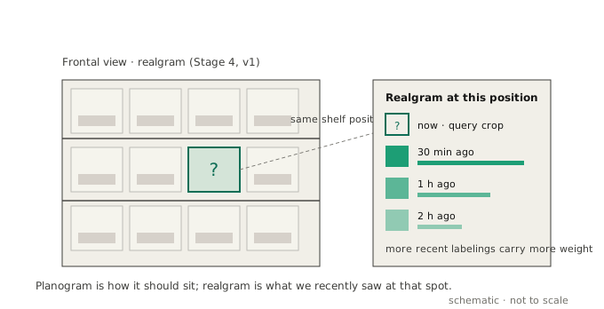
A crop does not live in a vacuum. It hangs at a fixed point on a shelf with regular recent labelings. That is a strong spatial and temporal signal that v0 ignores. We call it realgram, by analogy with planogram: a planogram is how it should sit, a realgram is what we recently saw there. Cosine similarity from the search space (how close two fingerprints point) is weighted by recency and by coordinate overlap. Accuracy moves to around 92%. Details in part one.

A shelf grid with one query cell marked unknown, linked to a panel listing what was recently labeled at the same shelf position, weighted so more recent observations count more. — The realgram weights candidates by what recently sat at the same spot, the more recent counting more.

v2: add tracking, around 94%

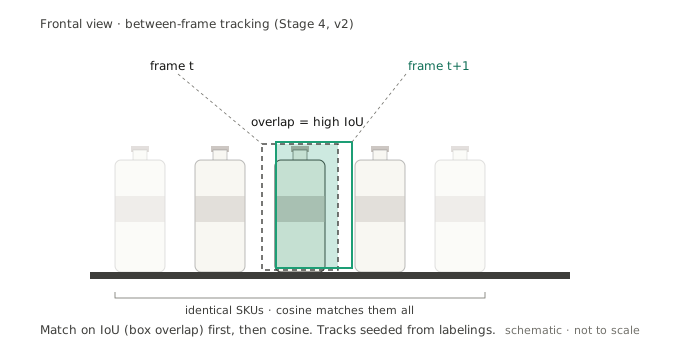
The pain is flicker. Across two neighboring frames the product did not change, yet the prediction jumps. That hurts OSA more than raw accuracy, because it generates phantom out-of-stock alerts. We fixed it with a modified DeepSORT (a tracker that follows each box from frame to frame). The original matches on embeddings first, which fails when ten identical bottles match everything. We match on IoU first (how much two boxes overlap), then cosine on top, and we seed tracks from labelings. Accuracy reaches around 94%. Details in part two.

A row of identical bottles with the tracked one carrying two boxes from consecutive frames that overlap heavily, showing the IoU used to link them before the visual match. — The box barely moves between frames. Matching on that overlap first stops the prediction from flickering.

v3: add a CatBoost ranker, around 96%

By the end of v2 there were 15 or more hand-tuned parameters and three candidate sources with scores that cannot be compared. We hand the choice to a table model. A CatBoostRanker (a tree model that ranks candidates) with a QuerySoftMax loss reads every feature of every candidate and learns to pick the winner. It reached around 96% on 49 features, including cross-frame features that brought flicker back down. Details in part three.

The classifier in one table

Version	What it adds	Solves
v0	ViT-Base-32, ArcFace, Qdrant nearest neighbor	Cold start on a drifting catalog
v1	realgram spatial-temporal context	Similar SKUs, bad light, turned packs
v2	modified DeepSORT tracking	Flicker between neighboring frames
v3	CatBoostRanker over 49 features	Incomparable scores, manual tuning

The remaining 4% are mostly meta-errors. Label mistakes poison the search space, knocked cameras zero out realgram, and new SKUs are not in the index yet.

What this overview leaves out

Two years held several hundred experiments, and most never shipped. They are collected in experiments that did not ship. The list runs through these: automatic search-space cleanup, super-resolution for price-tag OCR, a best-of-day composite frame, and OCR tag matching as a service. It also covers LLM and VLM features, planogram compliance by graph matching, stitching neighboring cameras, test-time augmentation, and a classical change detector.

Five things we took away

A drifting catalog beats a classifier every time. Do not train one classifier on 20,000 SKUs, because it breaks in the first week. Metric learning with nearest-neighbor search is the floor to build on.

Visual context alone is not enough. Any real retail setup needs a spatial signal, what sat on this shelf, and a temporal one, what sat there an hour ago. That is worth roughly seven points of accuracy.

Accuracy and flicker are different things. Business metrics like OSA and alert volume can drop while accuracy rises. Count flicker separately from day one.

Hand-glued heuristics stop scaling. Past about ten signal sources, a table ranker over the pipeline is where you end up. Plan for it.

Most of the last few points are meta-errors. Moving from 96% toward 98% is about labeling discipline, camera monitoring and new-SKU triage. The model is rarely the limit. The test phase of a shelf-monitoring pilot exists to measure all of this, in your stores, before anyone scales.