
A CatBoost ranker on top: one table replaces 15 parameters
This is part three of a series on recognizing products on supermarket shelves. The pipeline map gives the whole picture. Part one covers the embedder and realgram. Part two covers tracking.
By the end of part two we had an embedder, realgram and a modified DeepSORT, near 94%. We also had about 15 parameters tuned with Optuna, and three candidate sources whose scores cannot be compared. We replaced the heuristics with a CatBoostRanker on a QuerySoftMax loss. It learns to aggregate candidates from every source, plus a pile of context features. That reached around 96% on 49 features. It also broke the anti-flicker work, because tracking became one feature among many, and we got flicker back with 13 cross-frame features. Below, in order: why a table model fits this, how we trained it, and how the flicker came back and went out again.
Recap
We recognize about 20,000 SKUs from camera photos every 30 minutes. v0 detects crops with YOLO, then turns each into a numeric fingerprint (an embedding) with ViT-Base-32 and ArcFace. A nearest-match lookup in Qdrant, a vector database, lands near 85%. v1 adds realgram, the spatial and temporal context of what was recently labeled at a shelf spot, near 92%. v2 adds a modified DeepSORT, an object tracker that uses box overlap (IoU) first and embeddings on top. Its tracks are seeded from labelings, near 94% and half the flicker.
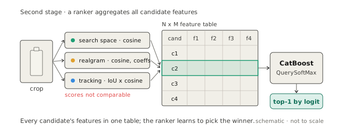
Three things were wrong. There were more than 15 parameters: about 10 in realgram and 5 in tracking, painful by hand, and the auto-tuner Optuna starts to overfit. The scores were a zoo: the embedder gives cosine, realgram gives cosine with coefficients, tracking gives IoU * cosine, with different scales and distributions. A 0.8 from one source and a 0.8 from another do not mean the same thing. And there were up to 20 candidates per crop, where the right one is usually present but the top-1 by any single score sometimes misses.
The obvious move is to hand the choice to a table model. Give it every feature of every candidate and let it learn.
What else can feed the model
Before picking a model, we listed every signal we could attach to a candidate. The table below is a solution space we explored. It is not a universal feature set. What actually helped is a separate discussion further down.
| Source | Example features | Why |
|---|---|---|
| Search space | max cosine, count in top-K, distance to nearest centroid | Visual similarity |
| Realgram | decay, overlap | Spatial and temporal context |
| Tracking | IoU, cosine, anchor flag | Neighboring frames hold the same items |
| Metadata | category, store, is_fresh | Narrows the space by business sense |
| Labelings | flag for presence in the last labeling, count in last 3 | The strongest signal lives in fresh labelings |
| Sizes | crop size in px and m, diff against the SKU size in the database | Shelf size should match the database |
| Price tags | does the nearest tag match the SKU price, is there a discount | Shelf price should match the database |
Hand-gluing all of that into a heuristic is a bad idea. The features are numeric or categorical, so the job fits a table boosting model cleanly.
Why ranking suits the problem
How we hand the task to the model decides whether we bake the brittle rules back in. The framing is a real decision, so it is worth a paragraph.
The natural thought is classification: pick one correct candidate out of N. But N differs per crop, from 1 to 20. Fixing the list length forces a rule for what to drop, which is the kind of heuristic we are trying to escape.
The cleaner framing is ranking with a binary target. Inside a group, which is one crop, one candidate is correct and the rest are wrong, and the group size is free. That narrows the library choice and fits the task exactly.
CatBoostRanker and QuerySoftMax
What this buys, in plain terms: the model learns the weighting we used to tune by hand, and keeps improving as we add features. The rest of this section is the how, for the technically curious.
The big table libraries all do ranking: LightGBM, XGBoost and CatBoost. We took CatBoost, for its wider set of ranking losses and because the team knew it well.
The loss is QuerySoftMax. In ordinary learning-to-rank the target is a position in an ideal list, first, second, third. We have no such order, only one correct class and the rest wrong. QuerySoftMax is essentially softmax with cross-entropy inside each group, normalized by group size. That fits a binary target in ranking.
Training it is ordinary CatBoost work: we set the usual knobs, the tree depth, the learning rate, the regularization, and let Optuna search over them. It runs on a GPU. We started near 100 features and trimmed to 36 with feature importance and SHAP, with no quality loss. SHAP scores how much each feature swayed a prediction. We weighed feature cost too: some need a scan over the whole search space, slow, and some are a plain database SELECT.
Pipeline v3
We leave the old pipeline running and stop asking it to make the call. It turns into an evidence gatherer. For each crop it still embeds the image, pulls the top candidates from Qdrant, runs realgram and runs tracking, exactly as before. What changes is how much we keep. Every source ends in a final score, and under that score sit all the smaller numbers that fed it. We take those too. Then we add the plain facts about the crop. Where it sits on the shelf, what was labeled here lately, how big it is, which category it falls in. Lay it all out and the crop becomes a small table: one row for each candidate, one column for each feature, up to twenty rows and a few dozen columns. The CatBoostRanker reads that table and scores every row. That score is called a logit, a raw confidence number, and the highest one wins.
Accuracy moved from around 94% to around 96%.
The bigger win is what it opened up. New features no longer need a pipeline rewrite. They are tested in the table. Over the following months we tried several hundred features. Most did not move quality, and reading why a feature failed turned out to be worth keeping.
Flicker came back, and how we removed it
We sat at 36 features with a flat metric for a while. Then we noticed flicker had risen well above v2.
The mechanics: in v2 the final prediction was almost always made by tracking. Tracking literally dragged the prediction from the previous frame onto the current one. In v3 tracking is one feature among many, and CatBoost decides looking at everything at once. The link to the previous frame weakened.
The flicker showed up as a class hopping between two similar SKUs on consecutive frames where nothing changed. Apricots reading as oranges. Tuna, sturgeon and butterfish trading places at the same spot.
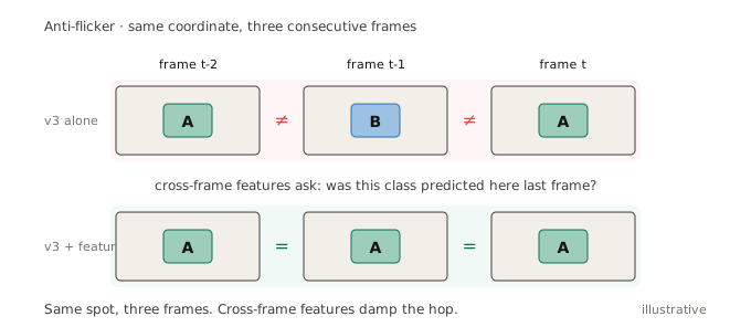
The fix is a set of 13 cross-frame context features, bringing the model to 49. Was this candidate predicted at these coordinates on the last frame, the last 3, the last 5? How many unique and total SKUs were predicted here over the last N frames? Is this candidate the most frequent here over the last N?
The effect: quality did not drop, which was the hard condition. Flicker fell by about 40% against v3 without these features. We came back near the v2 flicker level, now with CatBoost accuracy. By this point we had a small dataset to count flicker formally, plus a qualitative read on hard categories.
What did not work, and why
Several hundred features, mostly no effect. After each failure we tried to understand it. A few examples.
Size features: crop size in px and m, the diff against the database SKU size, a z-score of that diff against history. It helped in select cases, a 0.5 against a 1.5 liter bottle, 200 against 400 grams of peas. Mostly it was noise, because different flavors of one product have identical sizes, so the feature cannot break the tie.
Price-tag features: is the nearest tag recognized, what price, does it match the database, any discount. OCR is decent, though not everywhere, because some cameras have light and quality issues. Discounted prices are not always updated in the database. And the correct tag for a SKU can sit left, right, above or below, so the match itself is error-prone.
Embedding-geometry features: is this class centroid the nearest to the crop, what is the silhouette score when clustering the candidates. As hard as ArcFace tries to push look-alike products apart in the model’s memory, the fingerprints of similar SKUs stay similar. On UMAP, t-SNE and PCA views, the usual ways to plot these fingerprints in 2D, many classes overlap, and no geometry pulls them apart.
Where the last 4% live
Error analysis showed most of the remainder is meta-errors, independent of the pipeline.
Label mistakes. A labeler confirmed a visually similar but wrong class on a hard case. Those errors land in the metric through pre-labeling, in the search space, and in the CatBoost features, poisoning all three at once.
Knocked or moved cameras. Realgram zeroes out, and it is a strong feature, so every prediction on that camera sags until the context recovers.
New SKUs. They are physically absent from the search space, and the model cannot predict a class it never saw. How we found them and prioritized their labeling is a separate story.
What the series adds up to
We built the pipeline over more than a year, version by version: around 85%, then 92%, then 94%, then 96%, with rollbacks and rebuilds along the way.
Bare metric learning is only a starting point. Spatial context and cross-frame smoothing do the rest. On a hard CV task you cannot hand-glue about ten signal sources with a heuristic. Sooner or later you reach a table ranker over the pipeline. Accuracy and flicker are different things, and business metrics like on-shelf availability (OSA) and alert volume can sag while accuracy rises. Most errors at 96% are meta-errors, so moving toward 98% is labeling discipline and camera monitoring. The model is rarely the limit now.
If the path here looked too smooth, that is survivorship bias. The account of what failed is in experiments that did not ship. It covers super-resolution, VLM features, planogram compliance, stitching neighboring cameras, a change detector, and more. If you are scoping a build, the shelf-monitoring use-case is where this turns into a project.