Finding Cephalometric Landmarks in 3D CT Skull Scans
- Seed
- PoC
- MVP
- Production
- Chasing perfect
A 3D model that places the skull measurement points an orthodontist needs for treatment planning, the dozens of points they would otherwise mark by hand.
Where the data comes from
What we capture
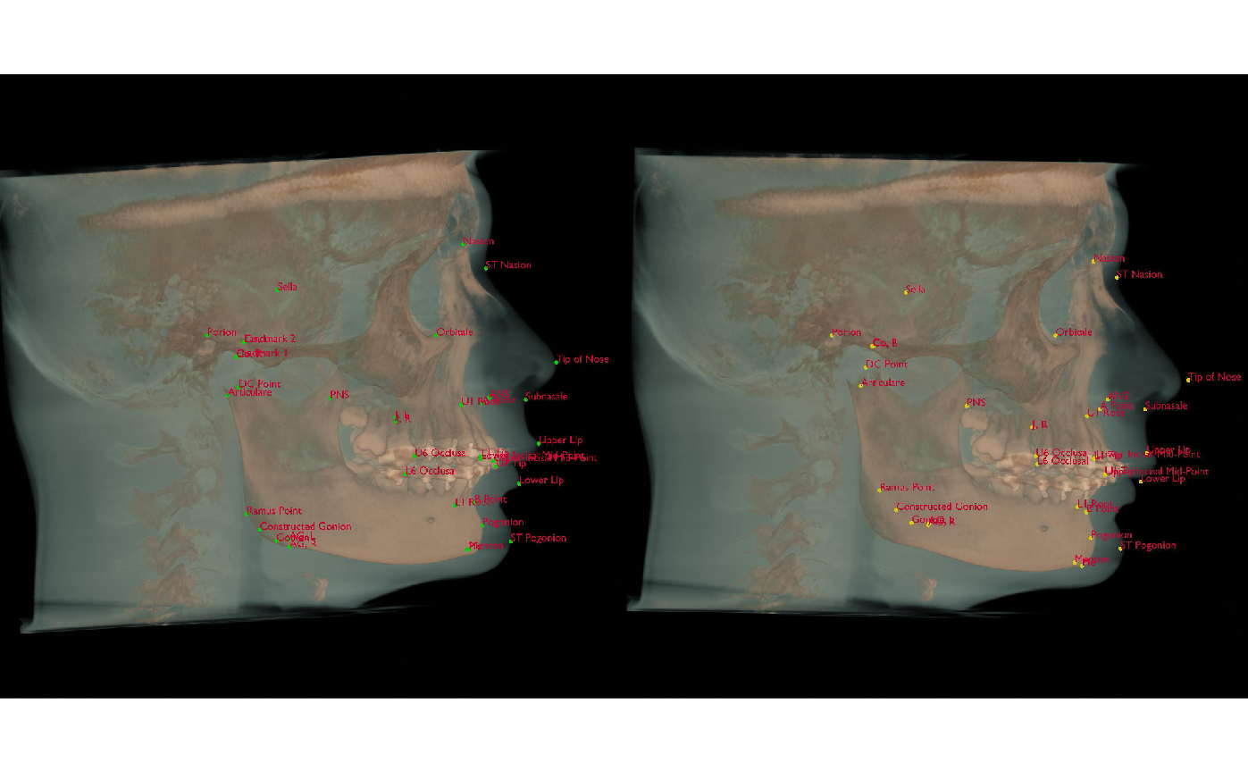
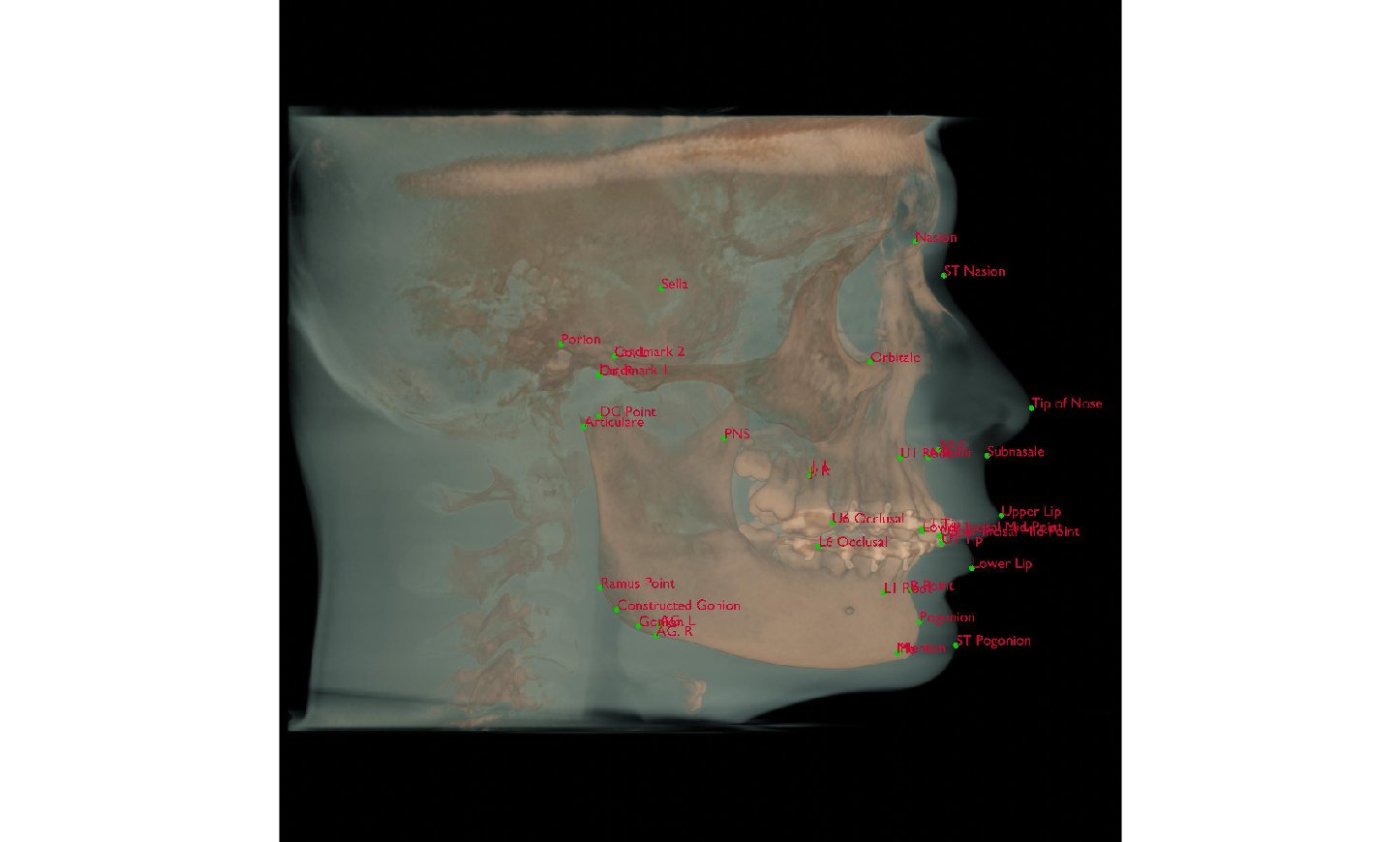
An orthodontic clinic plans treatment from CT scans of a patient's skull. Today a specialist opens each scan and marks dozens of measurement points by hand: cephalometric landmarks like Nasion, Sella and Gonion, the spots that fix the shape of the jaw and face. Marking them by hand is slow, and the result shifts from one person to the next.
What we get is one CT scan per patient: a stack of cross-section images in DICOM, the standard medical-imaging format. The scans vary in size, from about 461 by 461 by 346 up to 768 by 768 by 576 voxels (a voxel is one 3D pixel). Each scan also comes with the doctor's own marked points. We read those from the tool's own file, because the spreadsheet export drops the information about how the skull is turned in space.
What we do with it
How we train
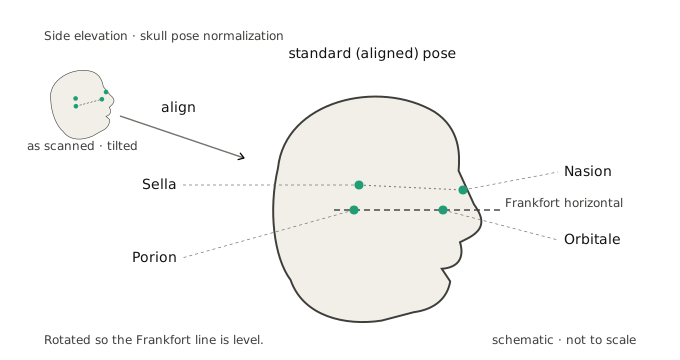
A model can only learn the landmarks if every skull is presented the same way, so the first job is to make the scans comparable. We put all the brightness values on the same medical scale (Hounsfield units, the standard scale for CT density) and squeeze them into a 0 to 1 range, so every scan looks the same to the model. Then we use four steady reference points (Porion, Orbitale, Nasion and Sella) to rotate each skull into one standard pose, and resize it to a fixed working size.
The model is a 3D version of ResNet, a well-proven image network, set up to predict all 36 point positions at once. We tried several sizes of it across many preprocessing settings and kept whatever placed the points closest to the doctor's, measured in voxels. The first version learned from only 84 scans. A later round used 805, with extra rotated copies of the scans added so the model sees more variety, a trick called augmentation.
- 01 Read the DICOM CT volume and put it on the Hounsfield scale
- 02 Read the doctors' annotations for the 36 ground-truth landmarks
- 03 Rotate the skull into one standard pose using four reference points
- 04 Normalize voxel values to 0-1 and resize the volume
- 05 Predict the landmark coordinates with a 3D ResNet
- 06 Measure the error in voxels against held-out scans
Stack
What comes out
How it performs
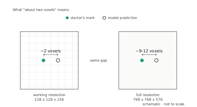
On scans it had never seen, the model places the 36 points close to where the doctor would, within about two voxels at its working size of 128 by 128 by 156. Two voxels is a small gap, about two grid steps on the working scan, so the marks land where a specialist expects on most scans. Training on the larger 805-scan set made it more accurate than the first try.
The model is strongest on common cases and drifts on rare ones, where it has few similar examples to learn from. So the lever now is more labeled scans. The model itself is not the limit. One caveat: error here is counted in voxels at the working size, so the same gap counts as more voxels on a full-size scan.